Time Complexities of the Most Important Algorithms in Programming and how to derive them

Time Complexity and Derivations of all the important Searching, Sorting, and Recursive Algorithms with diagrams and their comparisons

1. Searching Algorithms:

a. Linear Search:

- Time Complexity: O(n)

- Explanation: It sequentially checks each element in a list until the key element is found or the end of the list is reached. If the list contains n elements, the worst-case scenario occurs when the target element is at the end or not present at all, resulting in n comparisons.

b. Binary Search:

- Time Complexity: O(log n)

- Explanation: On sorted lists, binary search is an effective search algorithm. The target element and the middle element of the sorted list are first compared. When they match, the search is deemed successful. Otherwise, depending on whether the target element is smaller than or greater than the center element, the search moves to the left or right half. With each comparison, the process is repeated, halving the search space. The search space is halved at each step, resulting in an effective search, and this causes the logarithmic time complexity.

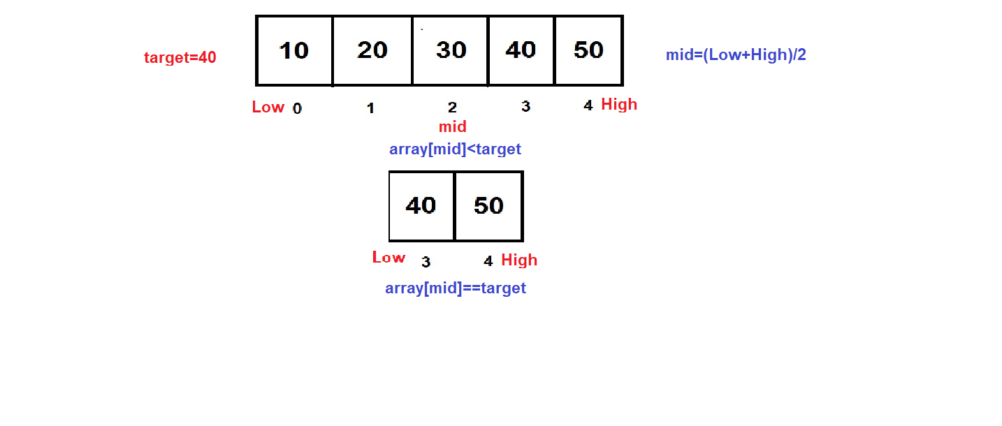
- Derivation:

The number of comparisons required in binary search can be derived by observing that the search space is halved at each step until the target element is found or the search space is exhausted.

At the first step, we have n elements.

At the second step, we have n/2 elements.

At the third step, we have n/4 elements.

...

At the kth step, we have n/(2^k) elements.

The search stops when n/(2^k) becomes 1, which occurs when 2^k = n. Taking the logarithm base 2 of both sides, we get k = log2(n). Therefore, the number of comparisons in binary search is O(log n).

2. Sorting Algorithms:

a. Bubble Sort:

- Time Complexity: O(n^2)

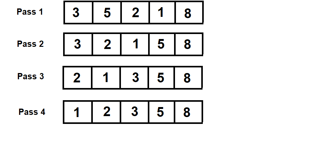
- Explanation: Bubble sort repeatedly compares adjacent elements and swaps them if they are in the wrong order. In each pass, the largest element bubbles up to the end of the list. This process is repeated until the list is sorted. The worst-case time complexity occurs when the list is in reverse order, and each element needs to be swapped with every other element.

- Diagram:

b. Insertion Sort:

- Time Complexity: O(n^2)

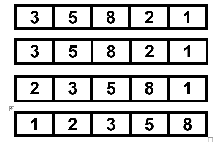
- Explanation: Insertion sort builds a sorted subarray by repeatedly inserting elements from the unsorted part into the correct position in the sorted part. It starts with a sorted subarray of size 1 and expands it by inserting the next element at the appropriate position. The worst-case time complexity occurs when the list is in reverse order, and each element needs to be compared and shifted for every element already sorted.

- Diagram:

Original unsorted list [5, 3, 8, 2, 1]:

c. Selection Sort:

- Time Complexity: O(n^2)

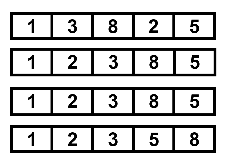
- Explanation: Selection sort picks the smallest element from the unsorted section repeatedly and replaces it with the unsorted part's initial element. It separates the list into an unsorted portion at the end and a sorted portion at the beginning. The smallest element from the unsorted section is chosen for each pass, and it is then relocated to the appropriate location in the sorted part. When the list is in reverse order and each element must be compared with every other element, the worst-case time complexity occurs.

- Diagram:

Original unsorted list [5, 3, 8, 2, 1]:

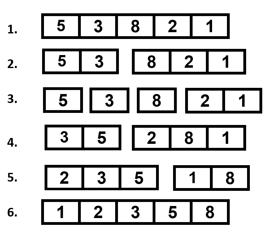
d. Merge Sort:

- Time Complexity: O(n log n)

- Explanation: Merge sort divides a list into two parts, recursively sorts those parts, and then combines the sorted parts to create the final sorted list. The list's partition into halves and the merging procedure give the time complexity. The list is split in half continuously until it is reduced to just one entry, at which point the sorted sublists are combined during the merging process.

- Diagram:

Original unsorted list [5, 3, 8, 2, 1]:

e. Quick Sort:

- Time Complexity: O(n log n) (average case), O(n^2) (worst case)

- Explanation: Quick sort chooses a pivot element, breaks the list into sublists around it, and then recursively sorts the sublists before and after the pivot. Elements that are less than the pivot are positioned before it, and elements that are larger than the pivot are positioned after it. The partitioning process dominates the time complexity. The pivot divides the list roughly in half at each level in the typical situation, adding complexity that takes O(n log n) time. The partitioning method only reduces the list size by one member at each level in the worst scenario, which results in O(n2) time complexity if the pivot is always the smallest or largest entry.

- Diagram:

Original unsorted list [5, 3, 8, 2, 1]: https://images.codingblocks.com/dsa/Screenshot%202023-07-15%20190940.png?

3. Recursive Algorithms:

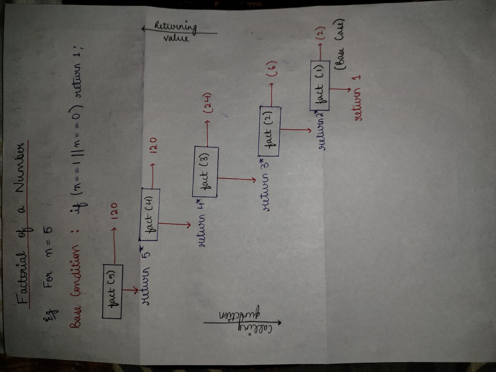
a. Factorial:

- Time Complexity: O(n)

- Explanation: The factorial algorithm calculates the product of all positive integers up to a given number. It can be implemented recursively by defining the factorial of 0 as 1 and the factorial of n as n multiplied by the factorial of (n-1). The recursive function calls itself until it reaches the base case of 0.

- Diagram:

b. Fibonacci Series:

- Time Complexity: O(2^n)

- Explanation: The Fibonacci series is a sequence of numbers in which each number is the sum of the two preceding ones. The base case is the Fibonacci of 0 as 0, the Fibonacci of 1 as 1, and the recursive case is Fibonacci of n as the sum of the Fibonacci of (n-1) and the Fibonacci of (n-2). The recursive function calls itself until it reaches the base cases of 0 and 1.

- Diagram:

fibonacci(6) = fibonacci(5) + fibonacci(4)

fibonacci(5) = fibonacci(4) + fibonacci(3)

fibonacci(4) = fibonacci(3) + fibonacci(2)

fibonacci(3) = fibonacci(2) + fibonacci(1)

fibonacci(2) = fibonacci(1) + fibonacci(0)

fibonacci(1) = 1

fibonacci(0) = 0

Therefore, fibonacci(6) = 5.