Searching Algorithms:

1. Linear Search:

- Space Complexity: O(1) (constant space)

- Description: A list or array's elements are iterated through in a basic method called linear search until the target element is found or the list's end is reached. It compares the first element to the target element from the beginning. The search is successful if they match. When a match is found or the end of the list is reached, the comparison process goes on to the next element. Beyond a few variables to keep track of indices and the target element, linear search doesn't need any extra room.

2. Binary Search:

- Space Complexity: O(1) (constant space)

- Description: An effective approach for searching in a sorted array is binary search. The target element and the middle element in the array are first compared. The search is successful if they match. The search moves to the left half of the array if the target element is smaller. The search moves to the right half of the array if the target element is greater. The search space is divided in half again, and the procedure is repeated until the target element is located or the search space is empty. Beyond a few variables to keep track of indices and the target element, binary search doesn't need any extra room.

Sorting Algorithms:

1. Bubble Sort:

- Space Complexity: O(1) (constant space)

- Description: Bubble sort repeatedly compares adjacent elements and swaps them if they are in the wrong order. Every element in the array is compared to its neighboring element starting at the beginning of the array. A switch is done if they are out of order. Up till the full array is sorted, this procedure is repeated. Bubble sort is an in-place operation, which means that it only needs the input array's available space.

2. Selection Sort:

- Space Complexity: O(1) (constant space)

- Description: Selection sort divides the array into a sorted portion and an unsorted portion. It switches the element at the start of the unsorted segment with the smallest element repeatedly from the unsorted portion. Up till the full array is sorted, this procedure is repeated. The input array is the only space needed for the selection sort to operate in place.

3. Insertion Sort:

- Space Complexity: O(1) (constant space)

- Description: Insertion sort builds a sorted portion of the array by iteratively inserting elements from the unsorted portion into their correct positions in the sorted portion. It begins by comparing the array's second member to the elements in the sorted section. The element is moved to the right to make room for the current element if it is smaller. Up till the full array is sorted, this procedure is repeated. The input array is all the space that is needed for insertion sort to work in-place.

4. Merge Sort:

- Space Complexity: O(n) (linear space)

- Description: Merge sort is a divide-and-conquer algorithm. The array is broken up into smaller subarrays until each subarray is made up entirely of one element. The subarrays are then combined by comparing and combining components in an ordered way. In order to store the temporary subarrays used during the merge operation, merge sort needs additional storage capacity. This extra space is typically allocated dynamically, resulting to an O(n) space complexity.

5. Quick Sort:

- Space Complexity: O(log n) to O(n) (varies depending on the implementation)

- Description: Quick sort is a divide-and-conquer algorithm that selects a pivot element and partitions the array into two subarrays: elements smaller than the pivot and elements larger than the pivot. It then recursively sorts the subarrays. Quick sort operates in-place, but the partitioning process requires additional space proportional to the size of the input. The space complexity ranges from O(log n) to O(n), depending on the implementation and partitioning approach.

Recursive Algorithms:

1. Fibonacci Series (Recursive):

- Space Complexity: O(n) (linear space)

- Description: The Fibonacci series is calculated recursively by summing the two preceding numbers in the series. Each recursive call creates a new stack frame, resulting in additional space proportional to the input size. As the depth of recursion grows linearly with the input size, the space complexity is O(n).

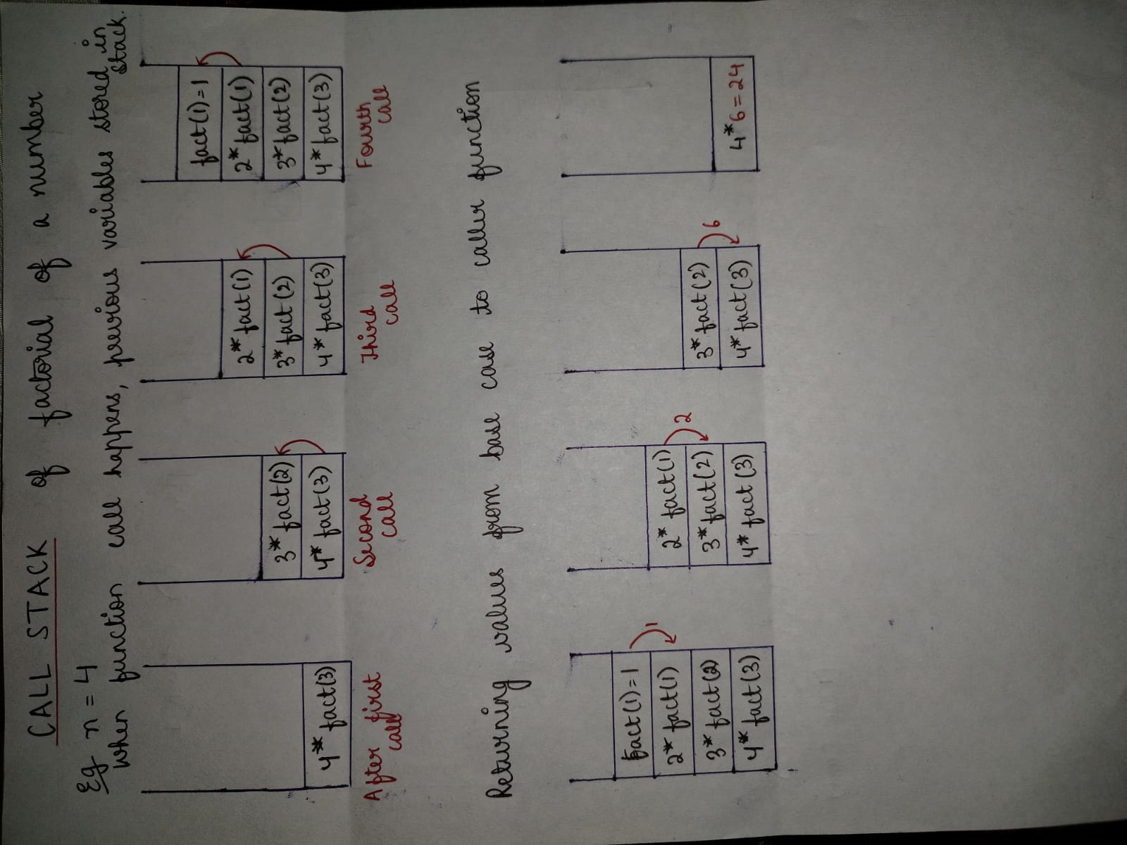
2. Factorial (Recursive):

- Space Complexity: O(n) (linear space)

- Description: Factorial is calculated recursively by multiplying a number with the factorial of its predecessor. Similar to the Fibonacci series, each recursive call creates a new stack frame, leading to linear space complexity as the depth of recursion grows with the input size.